Contrastive Predictive Coding - Learning Representations by Predicting the Future

Saturday. March 14, 2026 - 9 mins

What if a model could learn useful representations of speech, images, text, and game observations — all with the same objective, and zero labels? That is the promise of Contrastive Predictive Coding (CPC) [1], proposed by van den Oord et al. at DeepMind in 2018.

The key insight is deceptively simple: predict the future in latent space. Not the raw future — predicting raw pixels or audio waveforms requires expensive generative models. Instead, predict a compact representation of the future from the current context, and use a contrastive loss to make the task tractable.

Main Idea

The central hypothesis is that high-dimensional signals — audio, images, text — share a common structure: the present and the future are not independent. They share some underlying slow-varying latent variable. A phoneme in speech spans many timesteps. An object in an image spans many patches. The story in a book spans many sentences.

If you can build a model that correctly predicts which future representation is real versus randomly sampled, it must have learned to extract this shared latent structure. That extracted structure is the representation.

CPC formalizes this as a mutual information maximization problem. Given a context $c$ and a future observation $x$, the goal is to learn representations that maximize:

\[I(x; c) = \sum_{x,c} p(x, c) \log \frac{p(x|c)}{p(x)}\]

Rather than modeling $p(x \vert c)$ directly — which requires a full generative model — CPC estimates the density ratio $\frac{p(x \vert c)}{p(x)}$, which is all you need to maximize MI.

Architecture

Figure 1 in the paper shows the architecture clearly. It has three components:

Encoder $g_{enc}$: Maps raw input $x_t$ to a compact latent representation $z_t = g_{enc}(x_t)$. For audio, this is a strided CNN operating directly on the waveform. For images, a ResNet. The encoder compresses the input — discarding local noise, preserving global structure.

Autoregressive model $g_{ar}$: Summarizes the history of latents $z_{\leq t}$ into a single context vector $c_t = g_{ar}(z_{\leq t})$. In the paper this is a GRU. The context $c_t$ is the model’s summary of everything it has seen so far.

Scoring function $f_k$: A log-bilinear model that scores how compatible a future latent $z_{t+k}$ is with the current context $c_t$:

\[f_k(x_{t+k}, c_t) = \exp\left(z_{t+k}^T W_k c_t\right)\]

A separate $W_k$ is learned for each future step $k$, giving the model flexibility to express what to look for at different horizons. Note the similarity to the two-tower retrieval setup — $W_k c_t$ is effectively a query transformation of the context before taking the dot product with the future embedding.

InfoNCE Loss and Mutual Information

Both the encoder and autoregressive model are trained jointly using a loss the authors call InfoNCE. Given a set $X = {x_1, …, x_N}$ containing one positive sample from $p(x_{t+k} \vert c_t)$ and $N-1$ negatives from the marginal $p(x_{t+k})$:

\[L_N = -\mathbb{E}_X \left[ \log \frac{f_k(x_{t+k}, c_t)}{\sum_{x_j \in X} f_k(x_j, c_t)} \right]\]

This is the categorical cross-entropy of correctly identifying the true future sample among $N$ candidates — a multiple choice problem over the minibatch.

Why this works: density ratio estimation

The optimal $f_k$ that minimizes this loss satisfies:

\[f_k(x_{t+k}, c_t) \propto \frac{p(x_{t+k}|c_t)}{p(x_{t+k})}\]

This can be derived by writing out the optimal classifier $p(d=i \vert X, c_t)$ — the probability that sample $x_i$ was drawn from the conditional rather than the marginal:

\[p(d=i|X, c_t) = \frac{\frac{p(x_i|c_t)}{p(x_i)}}{\sum_{j=1}^{N} \frac{p(x_j|c_t)}{p(x_j)}}\]

This is exactly the form of equation 4 when $f_k$ equals the density ratio. Since any multiplicative constant cancels in the softmax denominator, the model only needs to learn the ratio up to a constant — which is tractable without a full generative model.

Connection to Mutual Information

The InfoNCE loss provides a lower bound on mutual information:

\[I(x_{t+k}; c_t) \geq \log(N) - L_N\]

This can be shown by substituting the optimal $f_k$ back into $L_N$ and applying the law of large numbers to the sum over negatives (which converges to $(N-1) \cdot 1 = N-1$ since $\mathbb{E}_{x \sim p(x)}\left[\frac{p(x \vert c)}{p(x)}\right] = 1$), followed by a simple algebraic inequality.

Two consequences follow directly:

Minimizing $L_N$ maximizes a lower bound on MI — the objective has a rigorous information-theoretic interpretation.
Larger $N$ gives a tighter bound — more negatives means a harder classification task and a better MI estimate. This is why in-batch negatives at scale matter.

Experiments

The same CPC framework is applied to four domains, with only the encoder and autoregressive architecture changed to suit each modality.

Audio

Encoder: 5-layer strided CNN on raw 16KHz waveform, downsampling factor of 160 (one vector per 10ms). Autoregressive model: GRU with 256-d hidden state. Predicts 12 steps (120ms) ahead.

Results on LibriSpeech with a linear classifier on top of frozen CPC features:

Method	Phone ACC	Speaker ACC
Random init	27.6	1.87
MFCC	39.7	17.6
CPC	64.6	97.4
Supervised	74.6	98.5

The same representation captures both phonetic content and speaker identity — two very different aspects of speech — learned without any labels.

Vision

For images there is no natural time dimension. The authors adapt CPC spatially: a 256×256 image is divided into a 7×7 grid of 64×64 overlapping patches. A ResNet-v2-101 encodes each patch independently. A PixelCNN-style row GRU then processes rows top-to-bottom, and the contrastive loss predicts patch representations in rows below the current context — “future” is redefined as spatially below.

CPC improved ImageNet top-1 unsupervised classification from 39.6% (prior state of the art) to 48.7% — a 9% absolute gain.

Natural Language

Sentence encoder (1D-conv + mean-pool) embeds each sentence to a 2400-d vector. GRU predicts up to 3 future sentence embeddings. Evaluated on five NLP benchmarks against skip-thought vectors — competitive performance at much lower training cost, with no word-level decoder required.

Reinforcement Learning

CPC is added as an auxiliary loss on top of a standard A2C agent in DeepMind Lab. No replay buffer — predictions adapt online to the changing policy. Performance improves in 4 out of 5 tasks after 1 billion frames. The one task that does not improve (lasertag) is purely reactive and requires no memory, which is consistent with CPC’s strength in extracting slow, temporally extended features.

Empirical Verification

To build intuition for the theoretical claims, consider a toy bivariate Gaussian. All four plots below are generated from this setup — no neural networks, no real data, just samples from a known distribution where we can verify every claim analytically.

\[\begin{bmatrix} c \\ x \end{bmatrix} \sim \mathcal{N}\left(0, \begin{bmatrix} 1 & \rho \\ \rho & 1 \end{bmatrix}\right)\]

The true MI has a closed form: $I(x;c) = -\frac{1}{2}\log(1 - \rho^2)$. With $\rho = 0.8$, this gives $I = 0.5108$ nats.

We can verify three claims empirically:

Claim 1 — MI lower bound holds: $\log(N) - L_N \leq 0.5108$ for all $N$. ✓ Verified for $N \in {2, 4, 8, …, 512}$.

Claim 2 — Bound tightens with $N$: Gap shrinks from 0.28 at $N=2$ to 0.008 at $N=512$. ✓

Claim 3 — $f_k$ converges to true density ratio: The true log density ratio for this Gaussian is:

\[\log \frac{p(x|c)}{p(x)} = \underbrace{\frac{\rho}{1-\rho^2}}_{w_1 = 2.222} \cdot xc \underbrace{- \frac{\rho^2}{2(1-\rho^2)}}_{w_2 = -0.889} \cdot x^2 + \text{const}\]

Training a parametric model $\log f(x,c) = w^\top [xc, x^2, x, 1]$ using only InfoNCE loss recovers $w_1 = 2.215$, $w_2 = -0.896$ — within 1% of the true values, with no direct supervision on the density ratio. ✓

The gradient that drives this convergence is:

\[\frac{\partial L_N}{\partial w} = -\frac{1}{B}\sum_{i=1}^{B}\left[\phi(x_{pos}, c_i) - \sum_j \text{softmax}(S_{i,j}) \cdot \phi(x_j, c_i)\right]\]

The true feature minus the expected feature under the model’s current distribution — gradient is zero exactly when the model assigns full probability to the positive, i.e., when it has learned the correct density ratio.

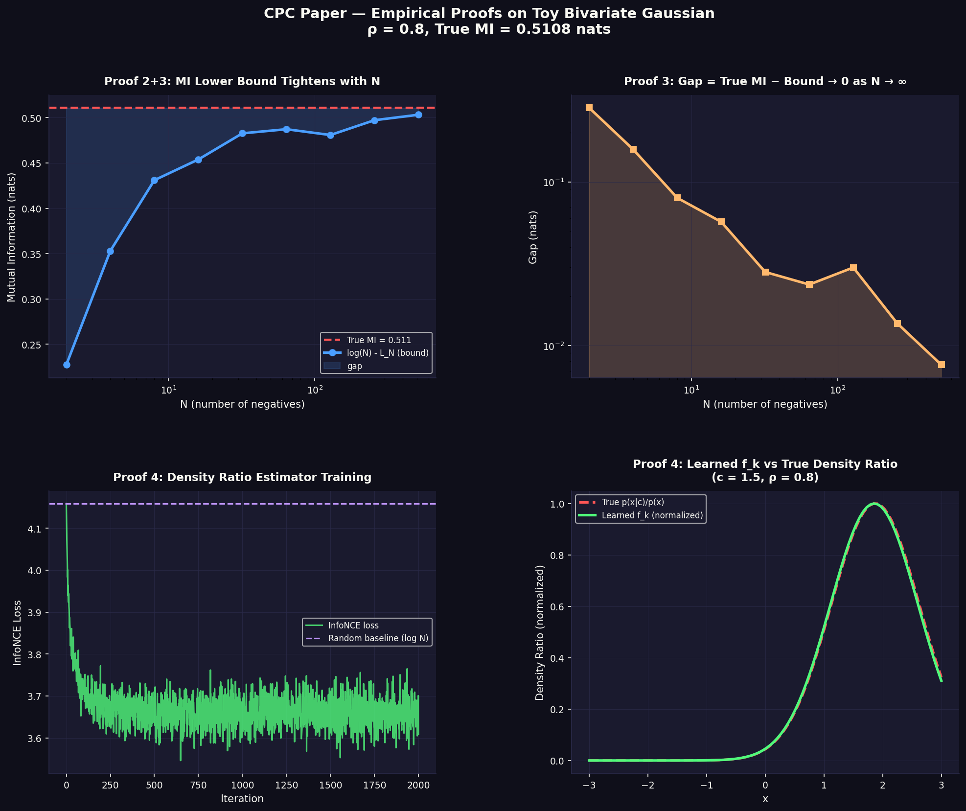CPC Empirical Proofs Four empirical proofs on a toy bivariate Gaussian ($\rho = 0.8$, True MI = 0.5108 nats). Top-left: MI lower bound $\log(N) - L_N$ approaches True MI as $N$ grows. Top-right: gap decays toward zero on a log-log scale. Bottom-left: InfoNCE loss during training of the density ratio estimator, converging well below the random baseline $\log N$. Bottom-right: learned $f_k$ (green) overlaid on the true density ratio $p(x|c)/p(x)$ (red dashed) — near-perfect recovery from contrastive training alone.

Discussion

Why not just do supervised learning? Supervised models are specialists — a phone classifier discards speaker information; a speaker classifier discards phonetic content. The same CPC representation achieves 64.6% on phones and 97.4% on speakers simultaneously. Labels are also expensive. Raw data is not.

The role of $N$: Larger $N$ means harder negatives, tighter MI bound, better representations. This is directly analogous to logQ correction in sampled softmax — more negatives with proper correction of the sampling distribution gives a better density ratio estimate.

Slow features: CPC naturally extracts features that span long time horizons. The ablation in Table 2 shows that predicting 2 steps gives 28.5% phone accuracy; predicting 12 steps gives 64.6%. Phonemes are slow features — they span ~100ms of audio. The multi-step prediction objective forces the model to capture them.

Universality: The same encoder-AR-InfoNCE skeleton works across audio, vision, text, and RL without domain-specific modifications. This is unusual — most representation learning approaches are modality-specific. CPC works because the underlying problem — extracting shared information between context and future — is universal.

Conclusion

CPC is a clean, principled framework for unsupervised representation learning. The key contributions are:

Framing representation learning as future prediction in latent space, avoiding expensive generative models
Deriving InfoNCE as a lower bound on mutual information, giving the objective a rigorous justification
Demonstrating the same framework works across speech, vision, text, and RL

This paper is also historically significant — it is a direct ancestor of wav2vec 2.0, data2vec, and the broader self-supervised pretraining paradigm that now dominates representation learning at frontier labs. Understanding it from first principles is worth the time.

References

Aaron van den Oord, Yazhe Li, Oriol Vinyals. Representation Learning with Contrastive Predictive Coding. arXiv:1807.03748, 2019.
Tomas Mikolov, Kai Chen, Greg Corrado, Jeffrey Dean. Efficient Estimation of Word Representations in Vector Space. arXiv:1301.3781, 2013.
Ryan Kiros et al. Skip-Thought Vectors. NeurIPS, 2015.
Michael Gutmann, Aapo Hyvärinen. Noise-Contrastive Estimation. AISTATS, 2010.
Ishmael Belghazi et al. MINE: Mutual Information Neural Estimation. ICML, 2018.