Graph Convolutional Nets - Basics
- 9 minsIntroduction
In recent times a lot of research and development have been made in geometric deep learning especially in the area of graph neural nets (GNN). Through GNNs we try to solve the predictive problem at hand using the native graph structure of the data rather than using tabular data structure. The breakthrough frameworks like GraphSage [1] and PinSage [2] which operates on the graph representation of the data and leverages node feature information to efficiently generate the node embeddings for previously unseen data. The PinSage algorithm also introduces highly efficient random walk techniques which increases the robustness of the learned model.
The field of geometric deep learning, GNNs in particular are applicable in massive scale recommender systems (eg. Pinterest), fake news detection, drug discovery and synthesis of chemical compounds, etc.
Current Methods and alternatives
Before diving into the nitty gritty details of graph convolutions and its inner workings we’ll discuss some alternatives to this methodology and what shortcomings they have.
MLP
Let us assume that we have a graph $G$ which can be represented by an adjacency matrix $A$. We can append the node features $F$ to the matrix $A$ and and train a MLP model on top each row to get some embeddings of the node based on a downstream task.
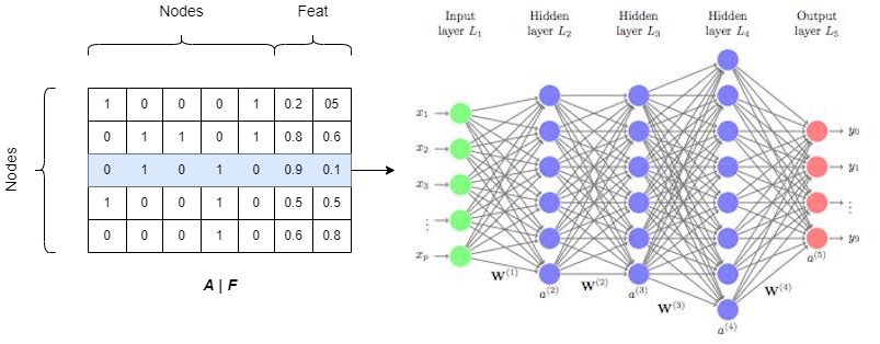
- Requires $O|V|$ parameters will lead to parameter explosion with increase in size of graph.
- Will not work with other graph of different size.
- It is sensitive to node ordering in the adjacency matrix.
Node2Vec
In the previous blog we discussed about the Node2Vec algorithm which uses Word2Vec algorithm used the hood. The major drawback of this algorithm is that its does not use the node features of the graph and only uses the adjacency matrix to create the node embeddings.
We’ll now take a brief look of how convolutions work and how it can be generalized to graph to address above shortcomings.
GCN
Convolutions
Under the hood, the main component of the GCNs are the graph convolutions. Convolutions are heavily used in computer vision algorithms. Through convolutions we can easily identify the unique spatial features of an image eg. the ears of human etc. The convolutional neural net consists of filter usually 3*3 matrix consisting of weights which convolve over the image taking the dot product of the image aggregating the inputs to accumulate the dominant features of the area the filter is convolving over.
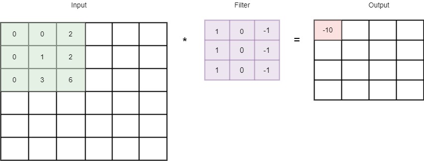
Convolution Filter to detect vertical edges
Single GCN Layer - Message Passing and Aggregation
Now that we know how a convolutions work aggregating the salient features of the image, we can now discuss how a single layer of GCN works. This is basically done in two steps -
- Message Passing - taking the features of the neighbouring nodes and passing it on to the current node in consideration.
- Aggregation - aggregating the neighbouring node features in an order invariant manner and concatenating it with the current node features.
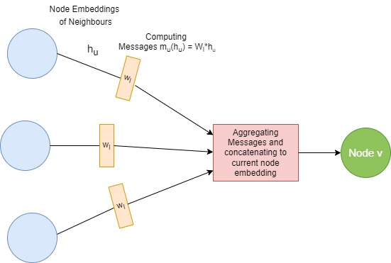
Single Layer of GCN
Let us assume -
- $h_v^l$ - current embedding $\forall$ node $v$ $\in$ $V$ at layer $l$
- $W_l$ - weight matrix to transform the embeddings of neighbouring nodes
- $B_l$ - weight matrix to transform the embeddings of current node
- $N_v$ - neighbouring nodes of current node $v$
- $\sigma$ - non linearity applied to calculated embeddings
Then the embedding of current node is calculated as -
\[h_v^{(l+1)} = \sigma(W_l\Sigma_{u \in |N_(v)|}{\frac{h_u^{(l)}}{|N(v)|}} + B_lh_v^{(l)})\]Here we have aggregated the neighbouring node embeddings by applying $SUM()$ operation we could have also used other order invariant operations like $MEAN()$, $MAX()$, $MIN()$, etc.
The node embeddings can be trained by any downstream task of our choice, one of the popular task is node classification.
Node Classification using GCNs
In an earlier blog regarding Node2Vec we created embeddings of nodes of Cora dataset which can be further used for classification. The Node2Vec algorithm did not use any info about the node features neither did it use the training node label information. Hence the embeddings generated were somewhat overlapping between the various classes.
We can improve upon the Node2Vec algorithm by using GCNs. We’ll implement it using PyTorch Geometric library.
Load the dataset and normalize the features
from torch_geometric.datasets import Planetoid
from torch_geometric.transforms import NormalizeFeatures

dataset = Planetoid(root='data/Planetoid', name='Cora', transform=NormalizeFeatures())

print('======================')
print(f'Number of graphs: {len(dataset)}')
print(f'Number of features: {dataset.num_features}')
print(f'Number of classes: {dataset.num_classes}')
Dataset: Cora():
======================
Number of graphs: 1
Number of features: 1433
Number of classes: 7
The dataset contains 1 graph with node features of 1433 dimensions distributed across 7 classes.
Lets create a two layer stacked GCN model.
from torch_geometric.nn import GCNConv
import torch.nn.functional as F

class GCN(torch.nn.Module):
    def __init__(self, hidden_channels):
        super().__init__()
        torch.manual_seed(1234567)
        self.conv1 = GCNConv(dataset.num_features, hidden_channels)
        self.conv2 = GCNConv(hidden_channels, dataset.num_classes)

    def forward(self, x, edge_index):
        x = self.conv1(x, edge_index)
        x = x.relu()
        x = F.dropout(x, p=0.5, training=self.training)
        x = self.conv2(x, edge_index)
        return x

model = GCN(hidden_channels=16)
print(model)
GCN(
  (conv1): GCNConv(1433, 16)
  (conv2): GCNConv(16, 7)
)
Train the classification model for 200 epochs .
model = GCN(hidden_channels=16)
optimizer = torch.optim.Adam(model.parameters(), lr=0.01, weight_decay=5e-4)
criterion = torch.nn.CrossEntropyLoss()

def train():
    model.train()
    optimizer.zero_grad()  # Clear gradients.
    out = model(data.x, data.edge_index)  # Perform a single forward pass.
    loss = criterion(out[data.train_mask], data.y[data.train_mask])  # Compute the loss solely based on the training nodes.
    loss.backward()  # Derive gradients.
    optimizer.step()  # Update parameters based on gradients.
    return loss

def test():
    model.eval()
    out = model(data.x, data.edge_index)
    pred = out.argmax(dim=1)  # Use the class with highest probability.
    test_correct = pred[data.test_mask] == data.y[data.test_mask]  # Check against ground-truth labels.
    test_acc = int(test_correct.sum()) / int(data.test_mask.sum())  # Derive ratio of correct predictions.
    return test_acc


for epoch in range(1, 201):
    loss = train()
    print(f'Epoch: {epoch:03d}, Loss: {loss:.4f}')
Epoch: 001, Loss: 1.9460
Epoch: 002, Loss: 1.9401
Epoch: 003, Loss: 1.9357
Epoch: 004, Loss: 1.9214
Epoch: 005, Loss: 1.9146
Epoch: 006, Loss: 1.9055
...
Epoch: 198, Loss: 0.3108
Epoch: 199, Loss: 0.3465
Epoch: 200, Loss: 0.3545
test_acc = test()
print(f'Test Accuracy: {test_acc:.4f}')
Test Accuracy: 0.8120
The test accuracy is better than the Node2Vec algorithm which gave 72.8% accurate results as opposed to 81.2% for GCNs.
Comparing the embeddings of the two models projected down to 2D space we see significant improvement for GCNs as compared to Node2Vec.
| Node2Vec Embeddings | GCN Embeddings |
|---|---|
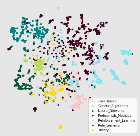 | 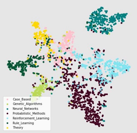 |
As we can see classes are much better segregated for GCN model.
Now there can be multiple ways we can generate and aggregate messages while convolving over neighbourhood edges e.g GraphSage algorithm concatenates the node information rather than summing it with neighbourhood nodes. We can also create an aggregation mechanism where we attend to the neighbourhood messages according to a predefined set of weights this method is known as Graph Attention Network (GAT) [3] details of which can be discussed in future blogs.
References
[1] William L. Hamilton, Rex Ying, & Jure Leskovec. (2018). Inductive Representation Learning on Large Graphs.
[2] Ying, R., He, R., Chen, K., Eksombatchai, P., Hamilton, W., & Leskovec, J. (2018). Graph Convolutional Neural Networks for Web-Scale Recommender Systems. Proceedings of the 24th ACM SIGKDD International Conference on Knowledge Discovery & Data Mining.
[3] Veličković, P., Cucurull, G., Casanova, A., Romero, A., Liò, P., & Bengio, Y. (2017). Graph Attention Networks. 6th International Conference on Learning Representations.