Imitation Learning - How to make it work?

Thursday. June 13, 2024 - 8 mins

One common blocker for learning policies for RL is setting up the environment itself. Another (suboptimal) technique that can be used to learn these complex tasks is imitation/behavior learning. In behavior learning, given a set of trajectories from the initial state to the goal, we’re trying to set up a supervised learning problem which learns the policy using the data provided.

There’s a key difference between the traditional supervised learning and imitation learning. In the traditional supervised learning, we assume that the data provided is independent and identically distributed (i.i.d) whereas in the case of imitation learning when we’re trying to learn a policy that is rarely the case. The current observation is directly a result of actions taken in the previous time steps. The process is “markov” at best.

Let’s take an example. Let us start at time , $t = 0$ , and we have an expert to traverse from our starting point to goal. At a given time $t$ we get an observation $o_t$ which is sampled from our training (expert) probability distribution $p_{\text{data}}(o_t)$. Using these trajectories, we’re trying to learn a policy $\pi_{\theta}(a_t | o_t)$ and imitate the trajectories of our expert while sampling from from test distribution $p_{\pi_{\theta}}(o_t)$ . Let’s say we train a sequential model which tries to learn our policy $\pi_{\theta}(a_t | o_t)$ from the expert data. There is a big drawback of such learned policies as a slight error any time step may lead to a huge deviation in our trajectory. As the new erroneous trajectory is not in our training set the model will give random results as we go to further time steps. This is depicted in the image below -

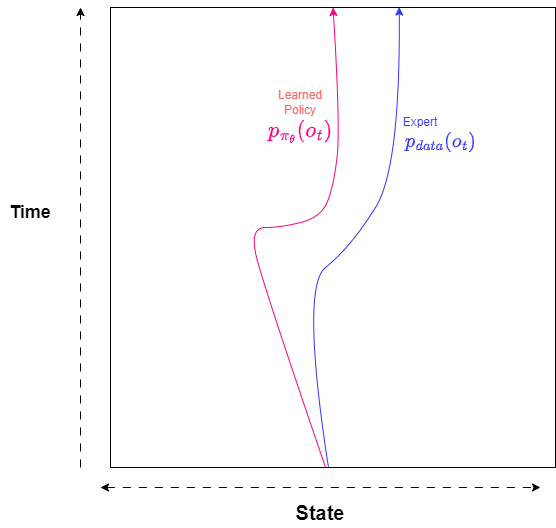
Imitation Learning Trajectory

Error Bound on Imitation Learning

Under certain assumptions it can be shown that the error in trajectories is bounded by square of time.

Let us assume that we have a cost function -

\[\begin{equation*} c(s_t, a_t) = \begin{cases} 0 &\text{$a_t \neq \pi^*(s_t)$}\\ 1 &\text{o/w} \end{cases} \end{equation*}\]

We also assume that our supervised learning algorithm learns the expert trajectories, s.t.

\(\pi_\theta(a \neq \pi^*(s)|s) \leq \epsilon \ \forall s \in D_{train}\) We can find the total expected cost under this assumption. Let $s \sim P_{train}(s)$ then \(E_{p_{train}(s)}[\pi_\theta(a \neq \pi^*(s)|s)] \leq \epsilon\) If for any time step $t$, $p_{data}(s_t) \neq p_{\theta}(s_t)$

The absolute error between the $p_{\theta}(s_t)$ and $p_{train}(s_t)$

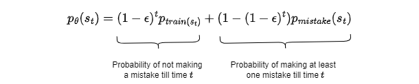
\(\begin{align*} |p_{\theta}(s_t) - p_{train}(s_t)| &= |(1 - \epsilon)^tp_{train(s_t)} + (1 - (1 - \epsilon)^t)p_{mistake}(s_t) - p_{train}(s_t)| \\ &= (1 - (1 - \epsilon)^t)|p_{mistake}(s_t) - p_{train}(s_t)| \\ \Sigma_{s_t}|p_{\theta}(s_t) - p_{train}(s_t)|&\leq 2(1 - (1 - \epsilon)^t) \leq 2\epsilon t \end{align*}\) The second last inequality comes from the total variational divergence upper bound between the two probability distribution. Now the expected value of cost for the entire trajectory is given by -

\(\begin{align*} \Sigma_{t} E_{p_\theta(s_t)}[c_t] &= \Sigma_{t}\Sigma_{s_t}p_{\theta}(s_t)c_t(s_t) \\ &\leq \Sigma_{t}\Sigma_{s_t}p_{train}(s_t)c_t(s_t) + |p_{\theta}(s_t) - p_{train}(s_t)|c_{max} \\ &\leq \Sigma_t (\epsilon + \epsilon t) \sim O(\epsilon T^2) \end{align*}\) $\therefore$ the maximum error that we can get is in the order of $O(\epsilon T^2)$

How to make Imitation Learning Work?

As we have seen in the previous section the error in the learned and the expert trajectories is of the order $O(\epsilon T^2)$, this error term explodes as we keep on increasing $T$.

There are various ways to mitigate this error -

• Be smart about how we collect the data and augment our training data accordingly.
• Train powerful models that make very few mistakes.
• Use multitask learning.
• Change the algorithm which learns the policy.

We’ll go over all the possibilities one by one -

1. Data Augmentation

In the paper, Bojarski et al [1], the authors solve self driving problems by using imitation learning. Apart from having a single camera, the authors have two extra cameras facing left and right respectively. If the car only learns from the front facing camera, it will start drifting from its trajectories as discussed in the previous section.

The left and right camera are used to store the augmented additional images which capture the shifts from the center lane. The annotations (actions) for these images are adjusted so that the car would course correct if it sees the same image during the testing phase.

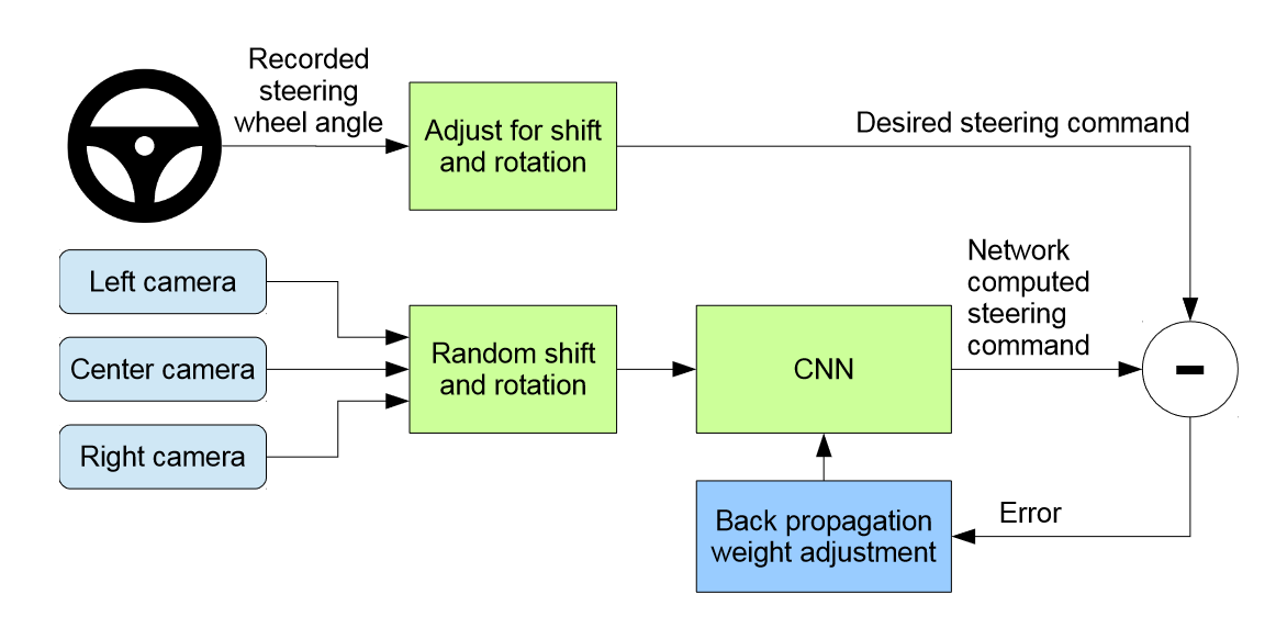
Data Augmentation for Self Driving Cars, figure from [5].

So retrospectively we’re better off augmenting the data with “unclean” samples that will help the agent learn to correct itself while in testing phase.

2. Training More Sophisticated Models

Often supervised models fail to predict the correct actions as they lack the capabilities to handle the complexity of the environment. For e.g. in the case depicted in the following image -

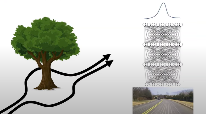
Single Modal Policy fails in complex tasks.

If we are outputting the continuous action space using a multivariate gaussian distribution. The distribution has single mode and the action predicted would be completely different from the ground truth. We can mitigate the issue by training more sophisticated models e.g. -

• Mixture of gaussians - We can train our neural net such that it outputs multiple gaussians with their respective weights i.e. $(w_i, \mu_i, \Sigma_i)$
• Latent Variable Models - Conditional Variational Autoencoders can be trained. These models generate the action spaces specific to the given conditioning variables. e.g. in the example above we can take the car’s current state and condition it on current state of the environment (e.g. tree present on the road) to generate the conditioned action spaces accordingly [2].
• Discretizing the action spaces - As we keep on increasing the dimensions of our action space, number of possible combinations of actions increases exponentially. Instead of predicting all the actions at ones, we can apply the strategy of predicting the actions autoregressively. For a $d$ dimensional action space we can train a sequential model as follows -

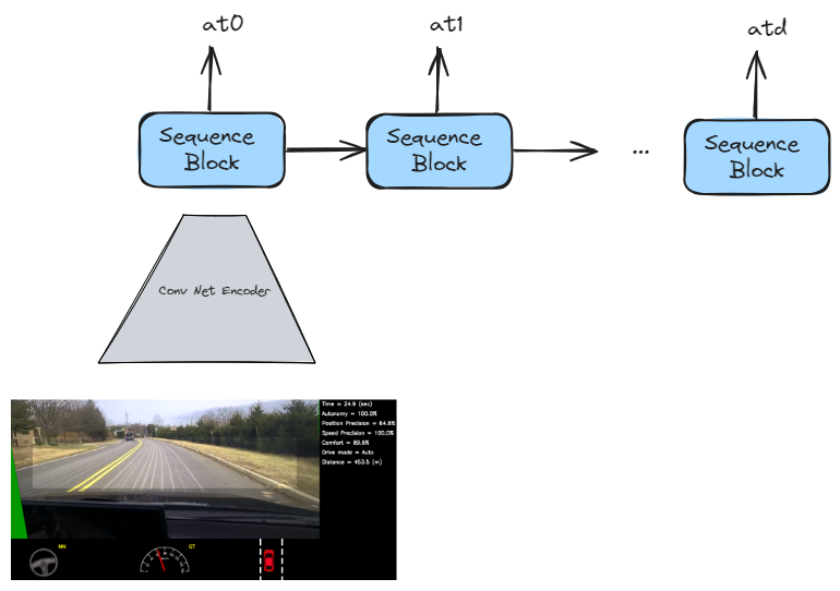
Autoregressive Action Prediction

Other methods include using diffusion models as well [3].

3. Multitask Learning

We can use multitask learning, which allows the model to learn multiple tasks simultaneously from the given data. Let’s say we have multiple demonstrations of trajectory reaching different final states for different demos. e.g.

\[\begin{align*} demo_1 &= \{s_1, a_1, s_2, a_2, ..., s_{t-1}, s_T\} \\ demo_2 &= \{s_1, a_1, s_2, a_2, ..., s_{t-1}, s_T\} \\ &... \\ demo_n &= \{s_1, a_1, s_2, a_2, ..., s_{t-1}, s_T\} \\ \end{align*}\]

Multitask Learning specifically goal conditioned behavior cloning [4] can be used to improve the performance of our model. Their are multiple benefits of the using such framework -

• Better utilization of the available data.
• The model can generalize to new goals that are not present in the training data.
• Can leverage imperfect demonstrations.

4. Changing the Algorithm

As discussed in the previous section when $p_{train}(o_t) \neq p_{\pi_{\theta}}(o_t)$ the expected error in the expert and learned policy is of the order $O(\epsilon T^2)$. We can change the data aggregation strategy to allow us to make $p_{train}(o_t) = p_{\pi_{\theta}}(o_t)$ using the DAgger (Dataset Aggregator) [5] algorithm.

Overall intuition of the algorithm is that we collect the training data from $p_{\pi_{\theta}}(o_t)$ instead of $p_{train}(o_t)$. We do so by running policy $\pi_{\theta}$ over multiple episodes.

1. Train $\pi_{\theta}(a_{t}|o_{t})$ from human data $\mathcal{D} = \{o_1, a_1, o_2, a_2, …, o_n\}$
2. Run $\pi_{\theta}(a_t|o_t)$ to get the data $\mathcal{D_{\pi}} = \{o_1, o_2, …, o_n\}$
3. Create a labeled data with action using human intervention $\mathcal{D}_{\pi} = \{o_1, a_1, o_2, a_2, …, o_n\}$
4. Augment the train data newly created data $\mathcal{D} \leftarrow \mathcal{D} \cup \mathcal{D}_{\pi}$ and repeat the process again.

Performing these steps over multiple iterations will ensure that $p_{train}(o_t) = p_{\pi_{\theta}}(o_t)$ and in that case it can be shown that error bound on the train and test trajectories is $O(\epsilon T)$.

The main bottleneck of the above methods is that we lack data to learn complex tasks, and we can compensate for that by simulating unlimited data from experience and have a reward model is place for correct actions taken. This is the fundamental concept of Reinforcement Learning and will be discussed in future blogs.

References

1. Mariusz Bojarski, Davide Del Testa, Daniel Dworakowski, Bernhard Firner, Beat Flepp, Prasoon Goyal, Lawrence D. Jackel, Mathew Monfort, Urs Muller, Jiakai Zhang, Xin Zhang, Jake Zhao, & Karol Zieba. (2016). End to End Learning for Self-Driving Cars.
2. Anthony Hu, Gianluca Corrado, Nicolas Griffiths, Zak Murez, Corina Gurau, Hudson Yeo, Alex Kendall, Roberto Cipolla, & Jamie Shotton. (2022). Model-Based Imitation Learning for Urban Driving.
3. Tim Pearce, Tabish Rashid, Anssi Kanervisto, Dave Bignell, Mingfei Sun, Raluca Georgescu, Sergio Valcarcel Macua, Shan Zheng Tan, Ida Momennejad, Katja Hofmann, & Sam Devlin. (2023). Imitating Human Behaviour with Diffusion Models.
4. Abhinav Jain, & Vaibhav Unhelkar. (2023). GO-DICE: Goal-Conditioned Option-Aware Offline Imitation Learning via Stationary Distribution Correction Estimation.
5. Ross, S., Gordon, G., & Bagnell, D. (2011). A Reduction of Imitation Learning and Structured Prediction to No-Regret Online Learning. In Proceedings of the Fourteenth International Conference on Artificial Intelligence and Statistics (pp. 627–635). PMLR.

Tweet Share

comments powered by Disqus