Node2Vec - Word2Vec in disguise (?)

Introduction

Traditional ml algorithms employ tabular data structure to solve a multitudes of supervised, unsupervised and semi-supervised problems ranging from image recognition, time series prediction, sentiment analysis, etc. Many problems like content recommendation have been attempted to solve using tabular data structure and have been known to beat SOTA benchmarks. In recent years a lot of focus from research community on using original graph structure of the data. Researchers from Pinterest have implemented GraphSage and PinSage content recommendation algorithms which beat the SOTA benchmark recommendation algorithms which use tensor decomposition techniques.

Before we dig into the complex algorithms like Graph Neural Networks and concepts like message parsing and distributed graph representation learning, we start off with two significant papers which set the foundation of GraphML. They are DeepWalk and Node2Vec. In particular we’ll be focussing on Node2Vec Algorithm and how it draws parallel to classic NLP model Word2Vec.

Word2Vec

Before we head into the Node2Vec model, lets look into the classic Word2Vec [1] algorithm from which it draws its parallel from. Word2Vec algorithm is used for generating vector representation of words taking into account the context (i.e. the words appearing in neighbourhood) in which the word appears. The two famous architectures used to by the algorithm are CBOW and Skipgram we’ll discuss the latter. Skipgram model is a single layer neural network model we predict the context (i.e. neighbourhood words) given the inputs words.

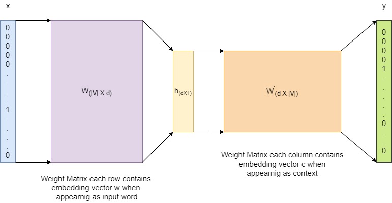
We provide one hot encoded word ($w$) vector $x$ as an input and predict the context ($c$) word $y$ from our training sample each iteration. Let the vector representation of $w$ be $v_{w}$ and that of $c$ be $v_{c}$.

We consequently formulate a supervised classification problem that predicts the probability of the context word given the input word using a softmax function i.e. -

Now lets say our corpus contains around $50k$ unique words and our projection layer is of 300 dimensions therefore size of weight matrix W is 50kX300 and W’ is 300X50K meaning at each iteration of training we update around 30M parameters which is computationally intensive and in some cases infeasible.

The word2vec paper addresses this issue and comes up with an efficient way to optimize the weights by changing the problem from calculating $p(c|w)$ to if the pair occurs together in the corpus. Now we’re essentially focusing on learning high quality embeddings rather than modelling the word distribution in the natural language. They formulate there problem by using a technique(/heuristic) known as negative sampling.

Now given a (word, context) pair the probability of (word, context) pair appearing together can be modelled by using a logistic regression classifier as follows -

$\therefore$ the probability of c not appearing in context of w is

Now for each positive sample (word, context), we randomly sample some negative examples for each input word i.e the words not appearing in the context of the w.

$\therefore$ the final objective function that we aim to optimise for skipgram model with negative sampling (SGNS) is

Where we have k negative samples for each positive samples. Which is computationally more efficient.

Node2Vec

Now that we have an overview of how Word2Vec algorithm works we can move forward with main topic of discussion Node2Vec [2]. To illustrate the workings of the algorithm we’ll investigate an open-sourced dataset known as Cora which consists of 2708 scientific publications classified into one of seven classes. There are directed links between two publications if one cited by the other i.e.

ID of cited paper --> ID of citing paper

The end goal is to come up with an embedding of the nodes (i.e. publications) of the graph and see if we can form clusters of different classes of publications without explicitly giving that information to the model.

We’ll be using PyTorch Geometric library to run the algorithm. Lets Load our data, torch geometric library comes pre-packaged with the Cora dataset so we can directly load from the library itself.

from torch_geometric.datasets import Planetoid
dataset = Planetoid(root = 'data/', name = 'cora')
print(f'Number of graphs in the data - {len_data}')
print(f'Number of classes in the data - {num_classes}')

Number of graphs in the data - 1
Number of classes in the data - 7

There is one graph in the dataset and the nodes are classified into seven different categories. Lets some of the statistics of the graph

data = dataset[0]
data

Data(x=[2708, 1433], edge_index=[2, 10556], y=[2708], train_mask=[2708], val_mask=[2708], test_mask=[2708])

The graph contains 2708 nodes each node can be represented by multi-hot encoded vectors containing info about the words in the publication. We wont be using these vectors for Node2Vec algorithm. There are 10556 directed edges. Lets initialise the Node2Vec algorithm using the given data.

Code for this blog is taken form here

import torch
from torch_geometric.nn import Node2Vec

device = 'cuda' if torch.cuda.is_available() else 'cpu'

model = Node2Vec(data.edge_index, embedding_dim=128, walk_length=20,
             context_size=10, walks_per_node=20,
             num_negative_samples=1, p=1, q=1, sparse=True).to(device) 

loader  = model.loader(batch_size = 128, shuffle = False, num_workers = 4)

Let’s go through all the parameters of the model one by one.

• data.edge_index - provides the the array of size (2, n_edges) where each row is a pair of node IDs having a directed edge between them
• embedding_dim - embedding dimension of the nodes
• walk_length - length of random walk from a given node
• context_size - length sliding window on a random walk to create training instances for the model
• walks_per_node - number of random walks per node
• num_negative_samples - number of negative samples for each instances, negative samples can be treated as fake random walks which are not actually present in the graph.

Node2Vec makes graph sequential via random walks, these random walks are biased with two parameters which controls whether the walk stays local (BFS) or explores (DFS) . They are -

• p - parameter of biased random walk, larger the p walk tends to explore more
• q - parameter of biased random walk, larger the q walk tends stay close to stating node

Let’s say we start from node t then the unbiased probability of going to neighbourhood node v is -

$\pi_{tv} = \text{transition probability from t to v}$

$Z = \text{Normalizing Factor}$

We can turn this into a biased second order RW by defining a search bias parameter $\alpha$.

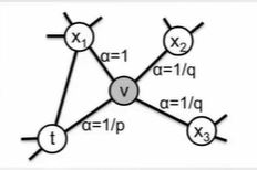
$\pi_{tx} = \alpha_{tx}*w_{tx}$

$d_{tx} = \text{distance between t and x}$

So if we set low value for parameter p the walk tends to stay local to starting node and so on e.g.

Biased Random Walk with high p and low q

Biased Random Walk with low p and high q

Now that we have initialised our model, we can go ahead and prepare sequences for Node2Vec and consecutively train the model. We can create a loader for the model that create sequences in batches -

loader  = model.loader(batch_size = 128, shuffle = False, num_workers = 4)
for idx, rw in enumerate(loader):
    print(rw[0].shape, rw[1].shape)
    break

torch.Size([28160, 10]) torch.Size([28160, 10])

The way PyTorch preprares the qequences is as follows - 
batch_size = 128
walks_per_node = 20
walk_length = 20
context_size = 10
total_walks_per_batch = (batch_size * walks_per_node) = 2560
num_sequences_per_rw = (walk_length - context_size + 1) = 11
num_seq_per_batch = (total_walks_per_batch * num_seq_per_rw) = 28160
for each sequence node 1 is the input and remaining nodes are context
and similarly for negative samples as well

Now lets train the model -

def train():
    model.train()
    total_loss = 0
    for pos_rw, neg_rw in tqdm(loader):
        optimizer.zero_grad()
        loss = model.loss(pos_rw.to(device), neg_rw.to(device))
        loss.backward()
        optimizer.step()
        total_loss += loss.item()
    return total_loss / len(loader)

# test function to evaluste the accuracy of the model
@torch.no_grad()
def test():
    model.eval()
    z = model()
    acc = model.test(z[data.train_mask], data.y[data.train_mask],
                     z[data.test_mask], data.y[data.test_mask],
                     max_iter=150)
    return acc

for epoch in range(1, 201):
    loss = train()
    acc = test()
    print(f'Epoch: {epoch:02d}, Loss: {loss:.4f}, Acc: {acc:.4f}')

100%|███████████████████████████████████████████████████████████████████████████████████| 22/22 [00:00<00:00, 35.56it/s]


Epoch: 01, Loss: 8.1546, Acc: 0.1820


100%|███████████████████████████████████████████████████████████████████████████████████| 22/22 [00:00<00:00, 34.34it/s]


Epoch: 02, Loss: 6.1120, Acc: 0.2160

...

100%|███████████████████████████████████████████████████████████████████████████████████| 22/22 [00:00<00:00, 39.94it/s]


Epoch: 199, Loss: 0.8245, Acc: 0.7280


100%|███████████████████████████████████████████████████████████████████████████████████| 22/22 [00:00<00:00, 40.34it/s]

Epoch: 200, Loss: 0.8255, Acc: 0.7280

Extracting the learned node embeddings from the trained model and projecting it down to two dimensions -

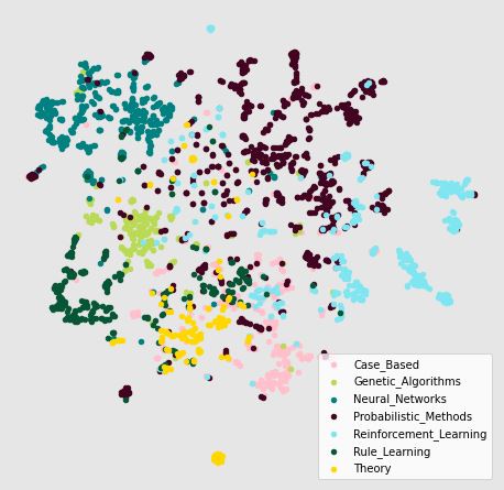
Note that we’ve not explicitly used the node labels in the model neither have we used the feature vector of the node, these embeddings are generated by simply using the citation network. Can we generate better embeddings by using the feature vector? (Spoiler Alert : We can, GNNs!!)

References -

[1] Tomas Mikolov, Ilya Sutskever, Kai Chen, Greg Corrado, & Jeffrey Dean. (2013). Distributed Representations of Words and Phrases and their Compositionality.

[2] Aditya Grover, & Jure Leskovec. (2016). node2vec: Scalable Feature Learning for Networks.

Tweet Share