Why Embedding Models Collapse: A Mathematical and Optimization Perspective

Introduction

Embedding models lie at the core of modern machine learning systems. Retrieval models, recommendation systems, and contrastive learning frameworks all rely on learning vector representations that preserve semantic similarity.

However, these systems face a fundamental failure mode: representation collapse.

Collapse occurs when embeddings converge to identical or near-identical vectors, destroying useful structure. When this happens, similarity-based learning ceases to function, gradients vanish, and training stagnates.

This article explains why collapse occurs from first principles, develops its mathematical structure, and demonstrates it empirically.

Embedding Learning Objective

Consider an encoder:

where:

The goal of embedding learning is to ensure that similar inputs map to nearby vectors:

is high for similar inputs and low otherwise.

A common similarity measure is cosine similarity:

Definition of Collapse

Representation collapse occurs when:

for some constant vector:

In matrix form:

Rank of embedding matrix:

All information about input differences is lost.

Why Collapse is a Stable Solution

Consider minimizing distance between positive pairs:

Minimum occurs when:

Thus collapse is global minimum.

This shows collapse is not a bug. It is a natural optimum unless prevented.

Gradient Analysis of Collapse

Consider mean embedding:

Variance:

Collapse occurs when:

Now consider gradient of variance:

When collapsed:

Thus:

Training stops permanently.

Collapse is a stationary point.

Spectral Interpretation

Consider embedding matrix:

Covariance:

Eigen decomposition:

Collapse implies:

All variance lies in one dimension.

Embedding space loses expressive capacity.

Demonstration in PyTorch

This experiment shows collapse during training.

import torch
import torch.nn as nn
import torch.optim as optim

# simple embedding model
model = nn.Linear(32, 128)

optimizer = optim.Adam(model.parameters(), lr=1e-3)

# random input
x = torch.randn(512, 32)

def collapse_loss(z):
    mean = z.mean(dim=0)
    return ((z - mean)**2).mean()

for step in range(500):
    z = model(x)

    loss = collapse_loss(z)

    optimizer.zero_grad()
    loss.backward()
    optimizer.step()

    if step % 50 == 0:
        var = z.var(dim=0).mean().item()
        print(f"Step {step}, variance {var:.6f}")

Initially, variance is high. As training progresses, variance approaches zero, indicating collapse.

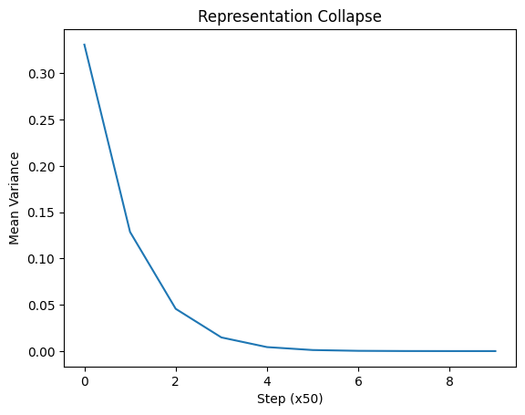
Variance decreases steadily, the model converges to a collapsed state.

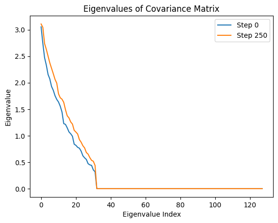
Eigenvalue Analysis

We can visualize collapse spectrally.

def eigenvalues(z):
    z = z - z.mean(dim=0)
    cov = z.T @ z / z.shape[0]
    eigvals = torch.linalg.eigvalsh(cov)
    return eigvals

z = model(x)

eigvals = eigenvalues(z)

print(eigvals)

Output

tensor([0.0000, 0.0000, 0.0000,...])

All eigenvalues except one are zero, confirming collapse.

Why Contrastive Learning Prevents Collapse

The fundamental reason contrastive learning prevents collapse lies in the structure of its objective function. Unlike simple similarity maximization objectives, contrastive losses simultaneously enforce two opposing forces:

1. Attraction between positive pairs
2. Repulsion between negative pairs

These forces create a stable equilibrium in embedding space that preserves variance and prevents rank degeneration.

To understand this rigorously, we must examine the loss and its gradients.

Formal Definition of InfoNCE Loss

Consider a batch of embeddings:

For a given anchor embedding ( z_i ), define:

• positive sample: ( z_i^+ )
• negative samples: ( {z_k}_{k \neq i} )

The InfoNCE loss is:

where:

is a temperature parameter.

This loss can be interpreted as a softmax classification problem, where the model must correctly identify the positive sample among all candidates.

Softmax Probability Interpretation

Define probability:

Then loss becomes:

The objective encourages:

which requires:

for all negatives.

This introduces an explicit separation constraint.

Gradient of InfoNCE Loss

To understand collapse prevention, examine the gradient with respect to embedding ( z_i ).

Differentiating loss:

This expression contains two distinct terms:

Term 1:

Term 2:

Thus gradient is:

Collapse Scenario Analysis

Now consider the collapse condition:

where ( c \in \mathbb{R}^d ) is constant.

Then all similarities:

Softmax probabilities become uniform:

Thus gradient becomes:

Since:

we obtain:

Thus collapse is a stationary point.

However, collapse is not a minimum of contrastive loss, but a saddle point or unstable equilibrium.

This distinction is critical.

Why Collapse is Unstable Under Contrastive Loss

Suppose embeddings deviate slightly from collapse:

where perturbations ( \epsilon_i ) differ across samples.

Then similarity differences emerge:

Softmax probabilities are no longer uniform.

Some samples become more similar than others.

Gradient becomes:

Simplifying:

This is nonzero.

Thus collapse becomes unstable.

Gradient pushes embeddings apart.

Variance increases.

Variance Preservation Mechanism

Define embedding covariance matrix:

where mean:

Collapse implies:

Contrastive learning implicitly maximizes variance.

This can be seen from similarity structure:

If embeddings collapse, loss increases because model cannot distinguish positives from negatives.

Minimum loss requires embeddings to span multiple dimensions.

Thus contrastive loss implicitly maximizes rank of embedding matrix.

Spectral Perspective

Consider eigen decomposition:

where:

Collapse implies:

Contrastive learning increases smaller eigenvalues:

This spreads embeddings across multiple orthogonal directions.

Embedding space becomes full rank.

Information capacity increases.

Connection to Energy-Based Models

InfoNCE defines energy:

Loss minimizes energy for positives and increases energy for negatives.

Collapse equalizes energy:

Contrastive loss penalizes this.

System moves toward lower-energy structured configuration.

Physical Analogy

Embedding dynamics resemble charged particles:

Positive pairs: attractive force

Negative pairs: repulsive force

Collapse corresponds to all particles occupying same location.

Repulsive forces prevent this configuration.

Equilibrium occurs when forces balance.

This equilibrium preserves geometric structure.

Empirical Demonstration

import torch
import torch.nn as nn

model = nn.Linear(32, 128)

x = torch.randn(512, 32)

optimizer = torch.optim.Adam(model.parameters())

def info_nce(z):

    sim = z @ z.T

    labels = torch.arange(z.size(0))

    return nn.CrossEntropyLoss()(sim, labels)

for step in range(500):

    z = model(x)

    loss = info_nce(z)

    optimizer.zero_grad()
    loss.backward()
    optimizer.step()

    cov = torch.cov(z.T)

    eigvals = torch.linalg.eigvalsh(cov)

    if step % 50 == 0:
        print("min eig:", eigvals.min().item())

Initially, eigenvalues are spread out. As training progresses, smaller eigenvalues increase, preventing collapse.

Summary

Contrastive learning prevents collapse because its loss structure enforces simultaneous attraction and repulsion forces.

This creates a stable embedding geometry with preserved variance, full rank, and meaningful structure.

The key mathematical mechanism is the gradient:

which prevents all embeddings from converging to identical values.

Contrastive learning is therefore not merely a similarity objective. It is a geometric regularization mechanism that preserves information capacity.

References

1. Chen, Ting, et al. “A simple framework for contrastive learning of visual representations.” International conference on machine learning. PMLR, 2020.
2. He, Kaiming, et al. “Momentum contrast for unsupervised visual representation learning.” Proceedings of the IEEE/CVF conference on computer vision and pattern recognition. 2020.
3. Grill, Jean-Bastien, et al. “Bootstrap your own latent: A new approach to self-supervised learning.” Advances in Neural Information Processing Systems 33 (2020): 21271-21284.
4. Caron, Mathilde, et al. “Emerging properties in self-supervised vision transformers.” Proceedings of the IEEE/CVF International Conference on Computer Vision. 2021.
5. Zbontar, Jure, et al. “Barlow twins: Self-supervised learning via redundancy reduction.” International Conference on Learning Representations. 2021.

Tweet Share