SimCLR - Learning Visual Representations Without Labels
- 10 minsSuppose you are tasked with building a product image search engine at an e-commerce company. You have millions of product images but almost no labels — no one has sat down and annotated which images are “electronics” or “footwear” or “home decor.” How do you learn useful representations of these images without labels?
The naive answer is: hire annotators. The better answer, increasingly, is: don’t use labels at all.
This is the setting contrastive self-supervised learning addresses. SimCLR [1], published by Chen et al. in 2020, presents a surprisingly simple framework that learns rich visual representations purely from unlabeled images — and comes close to matching supervised learning on ImageNet.
Main Idea
The core intuition is elegant. Take any image — say, a photo of a shoe. Crop two random patches from it, distort the colors of one, blur the other. Despite these transformations, both patches are still of the same shoe. A good visual representation should recognize this — the two views should map to nearby points in embedding space, while views from two completely different images should map far apart.
This is the contrastive prediction task: given one view, identify its paired view among all other views in the batch.
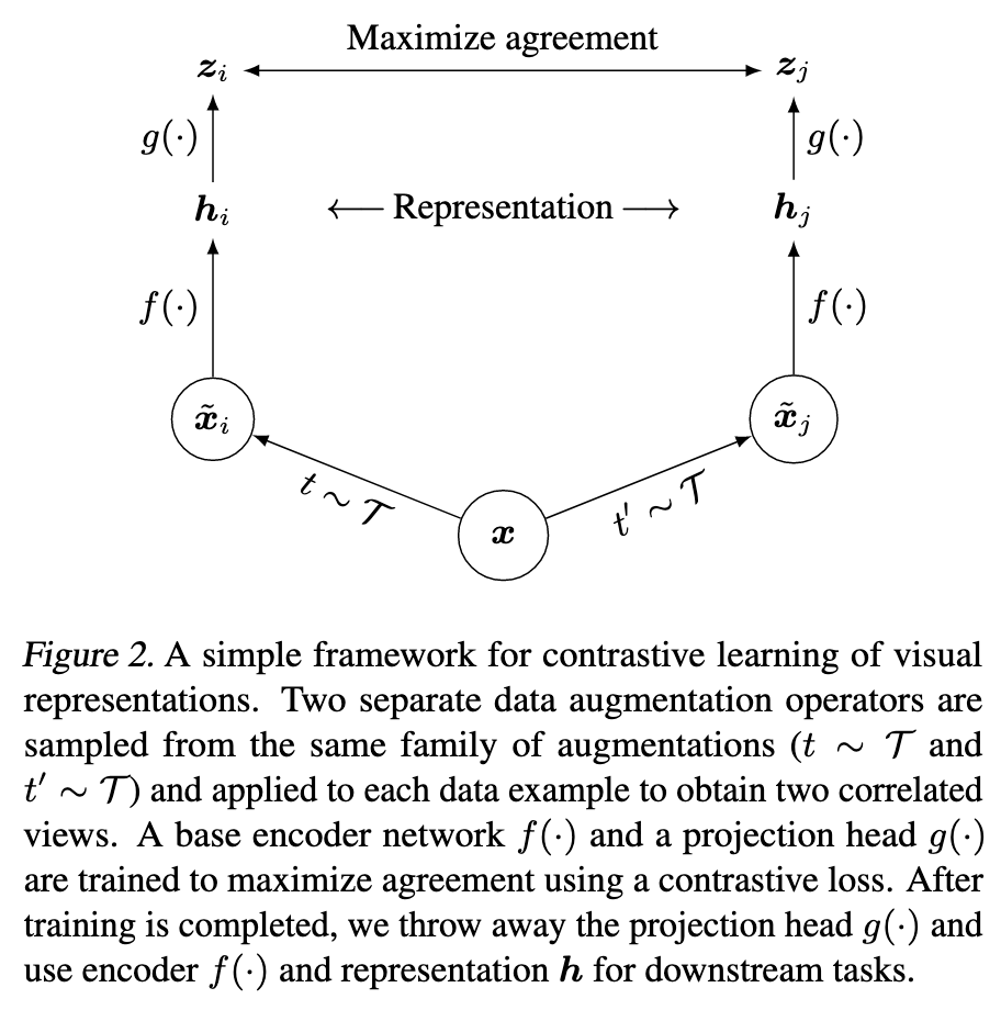
Figure 1: The SimCLR framework. Two augmented views of the same image are pushed together in embedding space, while views from different images are pushed apart.
Framework
SimCLR has four components:
1. Stochastic data augmentation — For each image $x$ in the batch, two random augmentations $t \sim \mathcal{T}$ and $t’ \sim \mathcal{T}$ are independently sampled and applied:
\[\tilde{x}_i = t(x), \quad \tilde{x}_j = t'(x)\]Both $t$ and $t’$ are drawn from the same augmentation family $\mathcal{T}$ — but they are independent draws, so the two views look different. The augmentation policy used in practice is: random crop + resize, random color distortion, random Gaussian blur.
2. Base encoder $f(\cdot)$ — A ResNet that maps augmented views to representation vectors:
\[h = f(\tilde{x}) = \text{ResNet}(\tilde{x}), \quad h \in \mathbb{R}^d\]3. Projection head $g(\cdot)$ — A small MLP that maps $h$ to a lower-dimensional space where the contrastive loss is computed:
\[z = g(h) = W^{(2)}\sigma(W^{(1)}h)\]where $\sigma$ is ReLU. This head is discarded after training — the representation $h$ is used for downstream tasks, not $z$.
4. Contrastive loss — NT-Xent (Normalized Temperature-scaled Cross Entropy), computed on the $\ell_2$-normalized projections $z$.
Contrastive Loss — NT-Xent
Given a batch of $N$ images, we obtain $2N$ augmented views. For any view $i$, its positive is its paired view from the same original image. The remaining $2(N-1)$ views in the batch serve as negatives — no explicit negative sampling is needed.
The loss for a positive pair $(i, j)$ is:
\[\ell_{i,j} = -\log \frac{\exp(\text{sim}(z_i, z_j)/\tau)}{\sum_{k=1}^{2N} \mathbf{1}_{[k \neq i]} \exp(\text{sim}(z_i, z_k)/\tau)}\]where $\text{sim}(u, v) = u^\top v / |u||v|$ is cosine similarity and $\tau$ is a temperature parameter. The final loss is averaged over all positive pairs $(i,j)$ and $(j,i)$ in the batch.
A few things to note here:
- $z$ is $\ell_2$-normalized before computing similarity, which keeps similarity scores bounded in $[-1, 1]$ and makes the temperature $\tau$ meaningful across training.
- Larger batch size $N$ directly means more negatives per positive pair — with $N = 4096$, each example sees $2(N-1) = 8190$ negatives. This is why larger batches help in contrastive learning, unlike supervised learning where the relationship between batch size and performance is more nuanced.
- At random initialization, when all embeddings are roughly uniformly distributed, the expected loss is $\log(2N - 1)$ — a useful sanity check.
Data Augmentation — The Most Important Component
Not all augmentations are equally useful. The paper systematically studies augmentations in pairs, and the result is striking: no single augmentation suffices to learn good representations, but composing augmentations dramatically improves quality.
The standout combination is random crop + random color distortion. Here is why this pair is special.
When you randomly crop two patches from the same image, both patches share nearly the same color distribution — the pixel histograms look almost identical. A neural network can exploit this shortcut to solve the contrastive task without learning anything meaningful: it just learns to match color histograms.
Color distortion breaks this shortcut. By randomly jittering brightness, contrast, saturation, and hue — and occasionally converting to grayscale — the two views no longer share a consistent color distribution. The network is forced to learn structural, semantic features instead.
This also explains why contrastive learning benefits from stronger color augmentation than supervised learning. Supervised learning is hurt by very aggressive color augmentation because color is a useful feature for classification. Contrastive learning benefits from it precisely because removing this shortcut forces better representations.
The Projection Head — Why You Should Use $h$, Not $z$
One of the more surprising findings in the paper is the role of the projection head $g(\cdot)$.
The projection head is a two-layer MLP placed on top of the encoder. The contrastive loss is computed on $z = g(h)$, not on $h$ directly. After training, $g(\cdot)$ is thrown away and $h$ is used for downstream tasks.
Why does this help? The contrastive loss forces $z$ to be invariant to the applied augmentations — it must map two very different-looking crops of the same image to nearby points. In doing so, $z$ discards information that is actually useful for downstream tasks, such as color and orientation. By inserting the projection head, this “invariance pressure” is absorbed by $z$, while $h$ retains richer information.
The paper verifies this directly. A separate MLP is trained to predict the augmentation applied to an image, using either $h$ or $z = g(h)$ as input:
| What to predict | $h$ | $z = g(h)$ |
|---|---|---|
| Color vs grayscale | 99.3% | 97.4% |
| Rotation | 67.6% | 25.6% |
| Original vs Gaussian noise | 99.5% | 59.6% |
$h$ retains substantially more information about the transformation applied — meaning $g(\cdot)$ successfully absorbs the invariances, leaving $h$ general.
In terms of linear evaluation accuracy on ImageNet:
- No projection head: ~53%
- Linear projection: ~60%
- Nonlinear projection (default): ~63%+
The difference between no projection and nonlinear projection is over 10% — for a component that is thrown away after training.
Hard Negative Weighting — Temperature as Implicit Mining
A key advantage of NT-Xent over other contrastive objectives (logistic loss, margin triplet loss) is that it automatically weights negatives by their difficulty, without any explicit hard negative mining.
Look at the gradient of NT-Xent with respect to the anchor embedding $u$:
\[\nabla_u = \left(1 - \frac{\exp(u^\top v^+/\tau)}{Z(u)}\right)\frac{v^+}{\tau} - \sum_{v^-} \frac{\exp(u^\top v^-/\tau)}{Z(u)}\frac{v^-}{\tau}\]where $Z(u) = \sum_k \exp(u^\top v_k/\tau)$ is the partition function.
The weight on each negative $v^-$ is $\exp(u^\top v^-/\tau) / Z(u)$ — a softmax weight. This is a competitive normalization: when one negative has a high similarity to the anchor, its weight dominates and easy negatives get suppressed toward zero.
To make this concrete, consider an anchor with these negative similarities:
| Negative | Similarity | NT-Xent weight ($\tau=0.5$) | NT-Logistic weight |
|---|---|---|---|
| Hard | 0.75 | 0.348 | 0.818 |
| Medium | 0.40 | 0.173 | 0.690 |
| Easy | 0.10 | 0.095 | 0.550 |
NT-Xent discriminates hard vs easy negatives at a 3.67x ratio. NT-Logistic (sigmoid-based) manages only 1.49x — the sigmoid saturates and cannot suppress easy negatives below ~0.5 even when they are far from the anchor.
The temperature $\tau$ controls the sharpness of this weighting:
| $\tau$ | Hard | Medium | Easy |
|---|---|---|---|
| 0.07 | 0.993 | 0.007 | 0.0001 |
| 0.1 | 0.969 | 0.029 | 0.001 |
| 0.5 | 0.565 | 0.281 | 0.154 |
| 1.0 | 0.449 | 0.316 | 0.234 |
At $\tau = 0.07$, almost all gradient mass concentrates on the single hardest negative — aggressive but potentially unstable if that negative is a false negative (a different crop of the same object category). At $\tau = 1.0$, the weighting is nearly uniform — hard negatives receive no special attention. The paper finds $\tau = 0.5$ works well on CIFAR-10, and around $0.1$ on ImageNet.
This is why loss functions like margin triplet loss require semi-hard negative mining — explicit, careful selection of which negatives to train on. NT-Xent handles this automatically through the partition function.
$\ell_2$ Normalization — Why It Matters for Retrieval
The contrastive loss is computed on $\ell_2$-normalized $z$ vectors. But what about the representation $h$ used downstream?
Consider an e-commerce retrieval setting. Two products have embeddings:
- Product A (semantically similar to query): $h = [3.0, 4.0, 0.1]$, magnitude $\approx 5.0$
- Product B (semantically different): $h = [5.0, 5.0, 5.0]$, magnitude $\approx 8.66$
Raw dot product with query $u = [0.6, 0.8, 0.02]$:
\[u \cdot h_A = 5.0, \quad u \cdot h_B = 8.66\]Product B ranks higher despite being semantically unrelated — its large magnitude dominates.
After $\ell_2$ normalization:
\[\text{sim}(u, h_A) = 1.00, \quad \text{sim}(u, h_B) = 0.82\]The semantically similar product now correctly ranks higher.
For linear evaluation (frozen encoder + linear classifier), $\ell_2$ normalization of $h$ has mixed effects — the linear layer can partially compensate for magnitude variation. But for ANN retrieval, normalizing $h$ before indexing is strongly recommended: it removes magnitude bias, makes dot product equivalent to cosine similarity, and is essentially free at inference time.
Results
A linear classifier trained on top of SimCLR representations achieves 76.5% top-1 accuracy on ImageNet (with ResNet-50 4×), matching a supervised ResNet-50 — without using any labels during pretraining. With only 1% of ImageNet labels for fine-tuning, SimCLR achieves 85.8% top-5 accuracy, outperforming AlexNet trained with 100× more labels.
Connection to Two-Tower Retrieval
The SimCLR framework maps naturally to two-tower models used in industrial retrieval systems. In SimCLR, the “two views” are two augmented crops of the same image. In a user-product two-tower model, the “two views” are a user and the product they interacted with — a positive pair by construction.
The same principles apply:
- NT-Xent / InfoNCE loss with in-batch negatives provides automatic hard negative weighting
- A projection head on top of each tower can absorb contrastive invariance pressure, leaving the tower output richer for downstream ranking
- $\ell_2$ normalization of tower outputs before ANN indexing removes magnitude bias from retrieval
- Larger batch sizes provide more negatives and a richer gradient signal — exactly the motivation behind systems like sampled softmax with logQ correction
The key difference is what constitutes “augmentation” — in image SSL, it is random crop and color jitter; in retrieval, it is the implicit diversity of user behavior and product catalogs. The mathematical framework is the same.
References
-
Ting Chen, Simon Kornblith, Mohammad Norouzi, Geoffrey Hinton. A Simple Framework for Contrastive Learning of Visual Representations. ICML 2020. arXiv:2002.05709
-
Aaron van den Oord, Yazhe Li, Oriol Vinyals. Representation Learning with Contrastive Predictive Coding. arXiv:1807.03748, 2018.
-
Kaiming He, Haoqi Fan, Yuxin Wu, Saining Xie, Ross Girshick. Momentum Contrast for Unsupervised Visual Representation Learning. CVPR 2020.
-
Florian Schroff, Dmitry Kalenichenko, James Philbin. FaceNet: A Unified Embedding for Face Recognition and Clustering. CVPR 2015.